The basic purpose of the aggregate demand and supply model is to recast the analysis of the real and monetary sectors in one diagram that explicitly isolates the average price level and real income.
The supply and demand sides of the economy together then determine the average price.
The AD-AS model overcomes major weaknesses in the traditional keynesian model in an inflationary context.
The aggregate supply (AS) curve is then added to represents the supply side of the economy and allows for disturbances and chain reactions to originate on the supply side.
Together the ASSR and AD curves simultaneously determine the short run equilibrium levels of real income and the average price level. Any disturbance will shift one or both the curves.
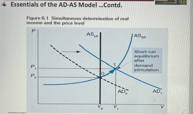
Simultaneous determination of real income and the price level
Aggregate demand relationship simply shows, for each price level, the aggregate quantity of goods and services demanded in the economy.
The AD curve shows all combinations of real income and the average price level at which there would be simultaneous equilibrium in the real and monetary sectors.
1) The interest rate effect : An increase in the average price, leads to a decrease in money supply, which increases interest rates and decrease expenditure.
2) The wealth effect : A higher average price level diminishes the real value of assets, people become affluent and expenditure decreases
3) The foreign trade effect : A higher domestic price level decreases export expenditure and encourages imports, so aggregate expenditure decreases.
4) The tax effect : When personal income increases in periods of inflation, taxpayers are pushed into higher personal income tax brackets. This decreases disposable income and expenditure.
5) The real income effect : A higher average price level lowers the real value of people's income and thus their capacity to spend.
The LM curve is always drawn for a particular constant price level. A higher price level implies a lower real money supply which shifts the LM curve left.
A higher price level implies a higher nominal value of transactions. This increases the nominal demand for money, for a given nominal money supply. This also shifts the LM curve to the left.

Deriving the AD curve from the IS-LM
To understand the steepness of the AD curve, the analysis relating to the factors affecting the potency of monetary policy is relevant.
1)Interest sensitivity of money. demand - if the money demanded is low, monetary contraction will have a large impact on the real economy. The AD curve will be flat.
2) Interest sensitivity of investment - If it is high, monetary contraction will have a large impact on the real economy. Therefore, for a given change in price, income will decline a lot, as a result the AD curve will be flat.
3) Size of the expenditure multiplier - If it is large, the drop in investment caused by monetary contractions will have a large impact on the real economy, as a result the AD curve will be flat.
Any non price stimulation of expenditure would cause the AD curve to shift to the right. Factors that contract expenditure would shift the AD curve to the left.
All internal factors and external factors that influence aggregate expenditure also influence aggregate demand.
Both expansionary fiscal policy and expansionary monetary policy would be reflected in the diagram as a rightward shift of the AD curve. Contractionary policy would shift the AD curve left. A surge in exports would shift the AD curve right.
Any change in the equilibrium level of Y, will shift the AD curve by exactly the same amount.
Policy potency
If fiscal policy is very potent, the AD curve will shift relatively far if an expansionary fiscal step occurs.
Likewise, if monetary policy is potent, the AD curve will shift relatively far when monetary expansion occurs.
Interest sensitivity of money demand, the income sensitivity of money demand, the interest sensitivity of investment and the size of the expenditure multiplier, any of these that make fiscal or monetary policy potent would lead to the AD curve shifting further.
The AS curve shows, for each price level, the aggregate level of real output Y that producers are willing or able to supply.
The supply side of the macro economy implies a constraint on the role of expenditure in determining the equilibrium level of real income and allows for independent supply side factors to impact on the economy.
Which factors determine aggregate supply ?
- Productivity of labor
- Exchange rate
- Cost of labor
- Cost of raw materials
- Cost of capital goods
The long run and the short run
The long run is when, following some disturbance, sufficient time has elapsed for any mistaken price expectation to have corrected itself so that the expected average price level is the same as the actual average price level.
The short run is when this has not yet happened, the expected average price level is not equal to the actual average price level.
Both the long run and short run aggregate supply curves show levels of output that producers are willing to supply.
The link between profit, output prices and input prices determines the level of output that producers are willing to supply.
How much producers supply will depend on the relationship between the prices that they can charge and their cost of production and how these vary over time.
The price setting relationship
The price setting relationship indicates how producers set their prices. The PS relationship assumes that prices are set as a mark up over wage cost, the producers determine the wage cost then adds a mark up on the set price of the goods.
(changes in non labor costs and taxes can impact the size of the mark up)
Note that the PS relationship assumes that producers are price setters and not price takers in goods markets.

Price setting relationship formula
Where P = price level
M = mark up
W = nominal wage level
Q = labor productivity
The wage setting relationship indicates how, on aggregate level, nominal wages are set. It is assumed that wages are not set in a competitive labor market.
Where W = nominal wage
Pe = expected price level
N = employment level
Z = institutional factors

Wage setting relationship formula

The wage setting and labor supply curves
Because the marginal productivity of labor decreases as a factor employs additional labor, Q is inversely related to the levels of employment N. Thus higher levels of employment N will be associated with lower levels of the implied real wage that firms are willing to pay as implied by the prices set by firms.
Graphically, the equilibrium levels of the real wage and employment are determined by the intersection of the PS and WS curves.
It implies that the real wage implicitly desired by workers during nominal wage setting must be equal to the real wage that firms are willing to pay

Price setting curve
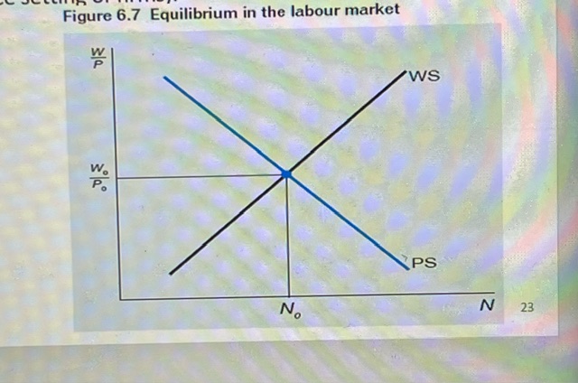
Equilibrium in the labor market
A shift of the PS curve, shows an increase in the mark up and will cause the price level to increase which in turn will cause the real wage that producers in effect are willing to pay at any employment level to decrease

A shift in the PS curve
A shift of the WS curve : will shift if any of the institutional factors that affect its position change. The power of labor unions and employer organisations, the payment of efficiency wages and unemployment and other benefits all influence the nominal wage level that workers are willing to work for.

A shift in the WS curve
The aggregate output produced by the number of workers employed in the long run equilibrium, this is shown by the intersection of the price setting and wage setting relationships. It represents the total amount of goods that producers in the economy can supply in the long run.
The relationship between the level of employment and the level of aggregate output can be depicted by the total production function for the economy. Total production is a function of the quantity of labor employed N, capital K and technology A.
Y = f (N ; K ; A)
Total production has a positive slope, the slope becomes flatter at higher levels of employment, as employment increases, output increases but at a decreasing rate. At some point the TP curve flattens out and reaches max. It means that even if more workers are employed, aggregate output will not increase
1) Seasonal unemployment - Occurs in seasonal patterns of increased or decreased activity in certain sectors of the economy.
2) Frictional unemployment - Which is always present, it exists because there is always a certain number of people who are in the process of searching for new jobs or busy changing jobs.
3) Cyclical unemployment - Exists because of short run cyclical downswings in the level of macroeconomic activity. As the level of Y fluctuates so does employment.
4) Structural unemployment - The form of unemployment that occurs regardless of the cyclical state of the economy. It is the most problematic and is difficult to analyse. Structural unemployment is involuntary unemployment.
The position of the ASLR curve is not constant or permanent. Changes in the structural and other factors underlie the position of the PS and WS curve and will influence the position of the ASLR curve.
The position of the ASLR is a variable over time. Any factor that reduces the equilibrium level of output in the PS WS diagram will be reflected as a leftward shift of the ASLR curve.
Changes from the price setting side can change the position of the ASLR curve at any time, while changes from the wage setting side occur only at wage bargaining time.

Shifts in the ASLR curve
The ASSR curve shows for each price level, the aggregate level of real output that producers are willing or able to supply.
In the short run producers can and probably will supply more or less than the long run equilibrium level of output if the actual prices and wages for a certain period allow for higher or lower profits.
Such opportunities occur when the actual prices set by producers, deviate from expectde prices due to some economic factor. ASSR, shows for each price level, the level of output Y that producers are willing to supply in the short run, as long as the price level deviates from the expected price level

Deriving the ASSR
When the ASSR curve shifts on its own, its intercept on the vertical ASLR line changes, it shifts up or down. When the ASSR shifts in lock steps with the ASLR the intercept on the vertical ASLR line does not change.
An increase in the expected price will shift the ASSR curve. The ASSR curve will shift left or right.

2 types of shifts in the ASSR
Every output level above or below the long run output level is the result of mistaken price expectations or price surprises, hence not sustainable. The only aggregate supply level that is sustainable in the long run, in the sense of being free of expectations.
Demand side disturbances leading to points off the ASLR curve.
Demand expansion : can be caused by expenditure stimulating events such as an increase in government expenditure, a tax cut, an exogenous increase in exports or a drop in imports.
Higher employment required to produce high output. This will reduce marginal product of labor. At the prevailing nominal wage, the unit cost of labor. Additional workers only employed if there is a higher price level, which will allow the real wage rate to fall and producers to recover the higher unit cost of production.
At a given nominal wage, the higher price level creates new profit opportunities.

Initial impact of demand expansion
The increase in the nominal wage increases production costs, which constrains the ability of producers to produce. Aggregate output contracts, the equilibrium moves up and to the left. There is a new pressure on the average price level, accompanied by a drop in the total production and income, we have an increasing price level combined with an economic contraction
Demand contraction : such a change can be caused by a decrease in government expenditure or a drop in exports due to a recession in the economies of our major trading partners.

demand contraction sequence
A supply shock affects both the long run and the short run aggregate supply relationship, a decrease in aggregate supply causes both ASSR and ASLR to shift to the left. Negative supply shock causes unemployment and inflation.
The short run equilibrium points slides up and to the left along the AD curve

Supply shock followed by supply adjustment

